Data Management
This section includes concepts and objects that operate on data. For oneDAL, such set of operations, or data management, is distributed between different stages of the data analytics pipeline. From a perspective of data management, this pipeline contains three main steps of data acquisition, preparation, and computation (see the picture below):
Raw data acquisition
Transfer out-of-memory data from various sources (databases, files, remote storage) into an in-memory representation.
Data preparation
Support different in-memory data formats.
Compress and decompress the data.
Convert the data into numeric representation.
Recover missing values.
Filter the data and perform data normalization.
Compute various statistical metrics for numerical data, such as mean, variance, and covariance.
Algorithm computation
Stream in-memory numerical data to the algorithm.
In complex usage scenarios, data flow goes through these three stages back and forth. For example, when the data are not fully available at the start of the computation, it can be done step-by-step using blocks of data. After the computation on the current block is completed, the next block should be obtained and prepared.

Data Management Flow in oneDAL
Key concepts
oneDAL provides a set of concepts to operate on out-of-memory and in-memory data during different stages of the data analytics pipeline.
Dataset
The main data-related concept that oneDAL works with is a dataset. It is a collection of data in a specific data format.
The dataset is used across all stages of the data analytics pipeline. For example:
At the acquisition stage, it is downloaded into the local memory.
At the preparation stage, it is converted into a numerical representation.
At the computation stage, it is used as one of the inputs or results of an algorithm or a descriptor properties.
Data source
Data source is a concept of an out-of-memory storage for a dataset. It is used at the data acquisition and data preparation stages to:
Extract datasets from external sources such as databases, files, remote storage.
Load datasets into the device’s local memory. Data do not always fit the local memory, especially when processing with accelerators. A data source provides the ability to load data by batches and extracts it directly into the device’s local memory. Therefore, a data source enables complex data analytics scenarios, such as online computations.
Transform datasets into their numerical representation. Data source automatically transforms non-numeric categorical and continuous data values into one of the numeric data formats.
For details, see dm data sources section.
Table
Table is a concept of in-memory numerical data that are organized in a tabular view with several rows and columns. It is used at the data preparation and data processing stages to:
Be an in-memory representation of a dataset or another tabular data (for example, matrices, vectors, and scalars).
Store heterogeneous data in various data formats, such as dense, sparse, chunked, contiguous.
Avoid unnecessary data copies during conversion from external data representations.
Transfer memory ownership of the data from user application to the table, or share it between them.
Connect with the data source to convert data from an out-of-memory into an in-memory representation.
Support streaming of the data to the algorithm.
Access the underlying data on a device in a required data format, e.g. by blocks with the defined data layout.
Note
For thread-safety reasons and better integration with external entities, a table provides a read-only access to the data within it, thus, table object is immutable.
This concept has different logical organization and physical format of the data:
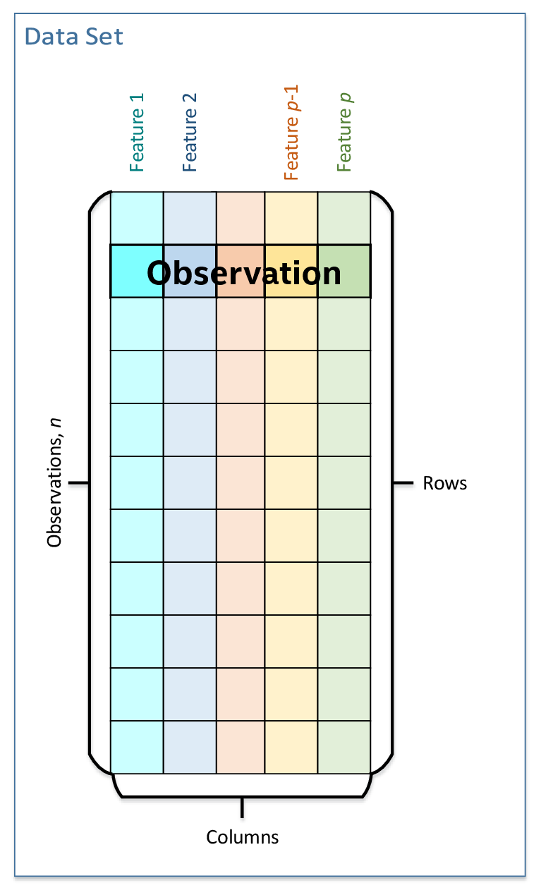
Logically, a table contains \(n\) rows and \(p\) columns. Every column may have its own type of data values and a set of allowed operations.
Physically, a table can be organized in different ways: as a homogeneous, contiguous array of bytes, as a heterogeneous list of arrays of different data types, in a compressed-sparse-row format. The number of bytes needed to store the data differs from the number of elements \(n \times p\) within a table.
For details, see dm tables section.
Table metadata
Table metadata concept provides an additional information about data in the table:
The data types of the columns.
The logical types of data in the columns: nominal, ordinal, interval, or ratio.
Only the properties of data that do not affect table concept definition is a part of metadata concept.
Accessor
Accessor is a concept that defines a single way to extract the data from a table. It allows to:
Have unified access to the data from table objects of different types, without exposing their implementation details.
Provide a flat view on the data blocks of a table for better data locality. For example, the accessor returns a column of the table stored in row-major format as a contiguous array.
Acquire data in a desired data format for which a specific set of operations is defined.
Have read-only access to the data.
For details, see dm accessors section.
Example of interaction between table and accessor objects
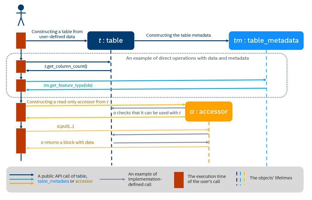
This section provides a basic usage scenario of the table and accessor concepts and demonstrates the relations between them. The following diagram shows objects of these concepts, which are highlighted by colors:
table object is dark blue
accessor is orange
table metadata is light blue

Sequence diagram of accessor-builder-table relations
To perform computations on a dataset, you have to create a table object first. It can be done either using a data source or directly from user-defined memory. The diagram shows the creation of a table object t from the data provided by user (not shown on the diagram). During a table creation, an object tm of table metadata is constructed and initialized using the data.
Once a table object is created, it can be used as an input in computations or as a parameter of some algorithm. The data in the table can be accessed via its own interface or via read-only accessor as shown on the diagram.
Graph
A graph is a concept of in-memory structured data that is organized as a graph with several vertices and edges. Graphs can be directed, undirected, weighted and attributed. Graphs are used at the data preparation and data processing stages to:
Be an in-memory representation of a dataset.
Store graph data in sparse data formats.
Avoid unnecessary data copies during conversion from external data representations.
Connect with the data source to convert data from an out-of-memory representation into an in-memory representation.
Note
For thread-safety reasons and better integration with external entities, a graph provides a read-only access to the data within it, thus, a graph object is immutable.
The logical organization of a graph and the physical format of the data are different:
Logically, a graph contains \(|V|\) vertices and \(|E|\) edges. All vertices of the graph are described with the same data type and respective operations on it. Similarly, the same is true for edges and attributes of the graph. The data types of vertices, edges, and attributes can be different.
Physically, the topology of a graph can be organized in CSR and others data formats.
For details, see dm graphs section.

